Discussion 4

Introduction

In this week’s discussion section, we will run and tune a KNN and Decision Tree model. We will see how our models perform differently, as well as attempt to improve them! Given the variables listed below, we are going to build our model to predict which National Park a given taxon is part of.

Data

Our data for this discussion section comes from a tidytuesday project. You can access the data on this google sheet and download as a CSV. The dataset contains National Park species obserations for the 15 most popular National Parks in the U.S. The user manual provided by the NPS cotains information on the different variables. Check out the table below with the different variables we will use this week.

Feature	Description
CategoryName	Broad taxanomic grouping
Order	Order of Species
Family	Taxanomic family
GRank	Global Rank, An assesment of the level of rarity or abundance of a taxon
ParkName	National Park Name
Sensitive	True/False variable on whether or not the taxon is sensitive
Nativeness	True/False variable on whether or not the taxon is native to the park
Abundance	Categorical variable specifying whether the taxons are rare, common, or abundant
Observations	The number of times the taxon has been observed

Time to dive in to our models!

1. Prepare the data

Read in the national park data and prepare your data from your models. We want our target variable to be ParkName, and all other variables in the table above to be our features. Then, split and scale the data.

import pandas as pd
import numpy as np
import matplotlib.pyplot as plt
import seaborn as sns
from sklearn.model_selection import train_test_split
from sklearn.neighbors import KNeighborsClassifier
from sklearn.tree import DecisionTreeClassifier
from sklearn.metrics import  accuracy_score
from sklearn.tree import plot_tree
from sklearn.preprocessing import StandardScaler

# Read in national park data
np_df = pd.read_csv('../data/national_park_species.csv')
np_df = np_df.drop(np_df.columns[0], axis=1)
pd.set_option('display.max_columns', None)
np_df.head()

	ParkCode	ParkName	CategoryName	Order	Family	TaxonRecordStatus	SciName	CommonNames	ParkAccepted	Sensitive	RecordStatus	Occurrence	OccurrenceTags	Nativeness	NativenessTags	Abundance	NPSTags	ParkTags	References	Observations	ExternalLinks	TEStatus	StateStatus	OzoneSensitiveStatus	GRank	SRank
0	ACAD	Acadia National Park	Mammal	Artiodactyla	Cervidae	Active	Alces alces	Moose	True	False	Approved	Present	NaN	Native	NaN	Rare	Resident	NaN	11	1	NaN	50	NaN	NaN	G5	ME: S5
1	ACAD	Acadia National Park	Mammal	Artiodactyla	Cervidae	Active	Odocoileus virginianus	Northern White-tailed Deer, Virginia Deer, Whi...	True	False	Approved	Present	NaN	Native	NaN	Abundant	NaN	NaN	20	0	NaN	50	NaN	NaN	G5	ME: S5
2	ACAD	Acadia National Park	Mammal	Carnivora	Canidae	Active	Canis latrans	Coyote, Eastern Coyote	True	False	Approved	Present	NaN	Non-native	NaN	Common	NaN	NaN	8	1	NaN	SC	NaN	NaN	G5	ME: S5
3	ACAD	Acadia National Park	Mammal	Carnivora	Canidae	Active	Canis lupus	Eastern Timber Wolf, Gray Wolf, Timber Wolf	True	False	Approved	Unconfirmed	NaN	Native	NaN	NaN	NaN	NaN	2	0	NaN	E	NaN	NaN	G5	ME: SH
4	ACAD	Acadia National Park	Mammal	Carnivora	Canidae	Active	Vulpes vulpes	Black Fox, Cross Fox, Eastern Red Fox, Fox, Re...	True	False	Approved	Present	NaN	Unknown	NaN	Common	Breeder	NaN	16	0	NaN	NaN	NaN	NaN	G5	ME: S5

# Encode categorical variables
for col in ['CategoryName', 'Order', 'Family', 'GRank', 'ParkName', 'Sensitive', 'Nativeness', 'Abundance','Observations', 'GRank']:
    np_df[f"{col}_cat"] = np_df[col].astype('category').cat.codes

# Split data into X and y
X = np_df[['CategoryName_cat', 'Order_cat', 'Family_cat', 'GRank_cat', 'Sensitive_cat', 'Nativeness_cat', 'Abundance_cat','Observations_cat', 'GRank_cat']]
y= np_df['ParkName_cat']

# Split data into training and testing
X_train, X_test, y_train, y_test = train_test_split(X,y, test_size = 0.33, random_state = 42)

# Standardize the predictors
scaler = StandardScaler() 
X_train_scaled = scaler.fit_transform(X_train)
X_test_scaled = scaler.transform(X_test)

2. Create a KNN Classifier

After running an untuned model, iterate over different values of K to see which performs best. Then, visualize how your accuracy changes wtih a varying K.

# Initialize KNN classiier
knn = KNeighborsClassifier()
knn.fit(X_train_scaled, y_train)
y_pred = knn.predict(X_test_scaled)

# Calculate accuracy
accuracy = accuracy_score(y_test, y_pred)
print(accuracy)

0.6029747149231532

### Tune a KNN Model and Visualize results
def knn():
    # Different k values to iterate over
    k_values = [3, 5, 7, 9, 11]
    accuracies = []

    # Create KNN model for each value of K, fit/predict, and calculate accuracies
    for k in k_values:
        knn = KNeighborsClassifier(n_neighbors=k)
        knn.fit(X_train_scaled, y_train)
        
        # Make predictions and calculate accuracy
        y_pred = knn.predict(X_test_scaled)
        accuracy = accuracy_score(y_test, y_pred)
        accuracies.append(accuracy)
        
        print(f"K={k} - Accuracy: {accuracy:.3f}")
    
    # Visualize K against accuracy
    plt.figure(figsize=(10,6))
    plt.plot(k_values, accuracies, marker='o')
    plt.xlabel('Number of Neighbors (K)')
    plt.ylabel('Accuracy')
    plt.title('KNN: Effect of K on Model Accuracy')
    plt.grid(True)
    plt.show()

knn()

K=3 - Accuracy: 0.593
K=5 - Accuracy: 0.603
K=7 - Accuracy: 0.600
K=9 - Accuracy: 0.600
K=11 - Accuracy: 0.597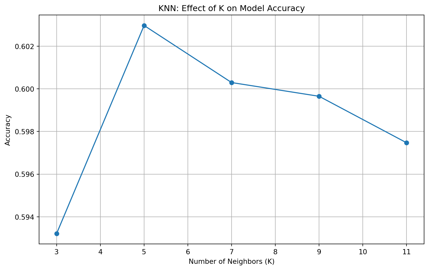

3. Create a Decision Tree

After running an untuned model, iterate over different max depths for your decision tree to determine which performs best. Then,create a decision tree visual using plot_tree. Lastly, find the most important features using .feature_importances_.

# Initialize Decision Tree classiier
dt = DecisionTreeClassifier()
dt.fit(X_train_scaled, y_train)
y_pred = dt.predict(X_test_scaled)

# Calculate accuracy
accuracy = accuracy_score(y_test, y_pred)
print(accuracy)

0.635746157659891

# Max depths to iterate over
max_depths = [2, 3, 4, 5]
accuracies = []

# Create decision tree model for different depths and report accuracies
for depth in max_depths:
    dt = DecisionTreeClassifier(max_depth=depth, random_state=42)
    dt.fit(X_train_scaled, y_train)
    
    # Make predictions and calculate accuracy
    y_pred = dt.predict(X_test_scaled)
    accuracy = accuracy_score(y_test, y_pred)
    accuracies.append(accuracy)
    
    print(f"Max Depth: {depth} - Accuracy: {accuracy:.3f}")

Max Depth: 2 - Accuracy: 0.466
Max Depth: 3 - Accuracy: 0.497
Max Depth: 4 - Accuracy: 0.532
Max Depth: 5 - Accuracy: 0.547

Visualize Models

# Create and fit model with best depth
dt_best = DecisionTreeClassifier(max_depth=5, random_state=42)
dt_best.fit(X_train_scaled, y_train)

# Create the mapping from numeric classes to descriptive names
class_mapping = dict(zip(dt_best.classes_, np_df.ParkName.unique()))

# Convert class labels in dt.classes_ to strings using the mapping
class_names_str = [class_mapping[cls] for cls in dt_best.classes_]

# Plot decision tree
plt.figure(figsize=(12, 15), dpi=700)
plot_tree(dt_best, feature_names=X.columns, class_names= class_names_str, 
          filled=True, rounded=True)
plt.title("Decision Tree Visualization (max_depth = 5)")
plt.savefig('decision_tree.png') 
plt.show()

Find important features

feature_importance = pd.DataFrame({
    'feature': X.columns,
    'importance': dt_best.feature_importances_
}).sort_values('importance', ascending=False)

print("\nFeature Importance:")
print(feature_importance)


Feature Importance:
            feature  importance
5    Nativeness_cat    0.705087
0  CategoryName_cat    0.126157
7  Observations_cat    0.092148
6     Abundance_cat    0.057482
1         Order_cat    0.009900
3         GRank_cat    0.008710
8         GRank_cat    0.000359
2        Family_cat    0.000159
4     Sensitive_cat    0.000000