# Import necessary libraries
import numpy as np
import pandas as pd
import matplotlib.pyplot as plt
from sklearn.model_selection import train_test_split
from sklearn.linear_model import Lasso, Ridge
from sklearn.metrics import mean_squared_error, r2_score
from ipywidgets import interact, FloatLogSlider

# Generate data
np.random.seed(42)
n_samples = 200
X = np.zeros((n_samples, 6))
X[:, 0] = np.random.normal(0, 1, n_samples)  # X1 - Important feature
X[:, 1] = np.random.normal(0, 1, n_samples)  # X2 -  Important feature
X[:, 2] = X[:, 0] + np.random.normal(0, 0.1, n_samples)  # Correlated with X1
X[:, 3] = X[:, 1] + np.random.normal(0, 0.1, n_samples)  # Correlated with X2
X[:, 4] = np.random.normal(0, 0.1, n_samples)  # Noise
X[:, 5] = np.random.normal(0, 0.1, n_samples)  # Noise

y = 3 * X[:, 0] + 2 * X[:, 1] + 0.5 * X[:, 2] + np.random.normal(0, 0.1, n_samples) Introduction
In this week’s discussion section, we will create some interactive plots to better undertsand how lasso and ridge regression are at work. To do so, we will use synthesized data that is made with the intention of better understanding how ridge and lasso regression are different based on the relationship of your parameters. It is important to note that your results with real data may look very different - unlike this notebook, the real world data you will be working with was not made to better understand regression models.
Data Loading
Copy the code below to load the neessary libraries genereate the data we will use. Read the comments to on each feature to get an idea of the relationship between variables.
Regression
Now that you have your data, do the following:
- Split your data into training and testing.
# Split data into training and testing sets
X_train, X_test, y_train, y_test = train_test_split(X, y, test_size=0.3, random_state=42)- Create and fit a ridge regression
# Create and fit Ridge regression model
ridge_model = Ridge()
ridge_model.fit(X_train, y_train)
ridge_predictions = ridge_model.predict(X_test)- Calculate the MSE and \(R^2\) for your ridge regression.
# Calculate MSE and R^2 for Ridge regression
ridge_rmse = np.sqrt(mean_squared_error(y_test, ridge_predictions))
ridge_r2 = r2_score(y_test, ridge_predictions)
print("Ridge Regression RMSE:", ridge_rmse)
print("Ridge Regression R²:", ridge_r2)
Ridge Regression RMSE: 0.14410020171824725
Ridge Regression R²: 0.9984722762470866- Create and fit a lasso model.
# Create and fit Lasso regression model
lasso_model = Lasso()
lasso_model.fit(X_train, y_train)
lasso_predictions = lasso_model.predict(X_test)- Calculate the MSE and \(R^2\) for your lasso model.
# Calculate RMSE and R^2 for Lasso regression
lasso_rmse = np.sqrt(mean_squared_error(y_test, lasso_predictions))
lasso_r2 = r2_score(y_test, lasso_predictions)
print("Lasso Regression RMSE:", lasso_rmse)
print("Lasso Regression R²:", lasso_r2)
Lasso Regression RMSE: 1.2984978990079017
Lasso Regression R²: 0.8759496036905758Visualizing Ridge vs Regression
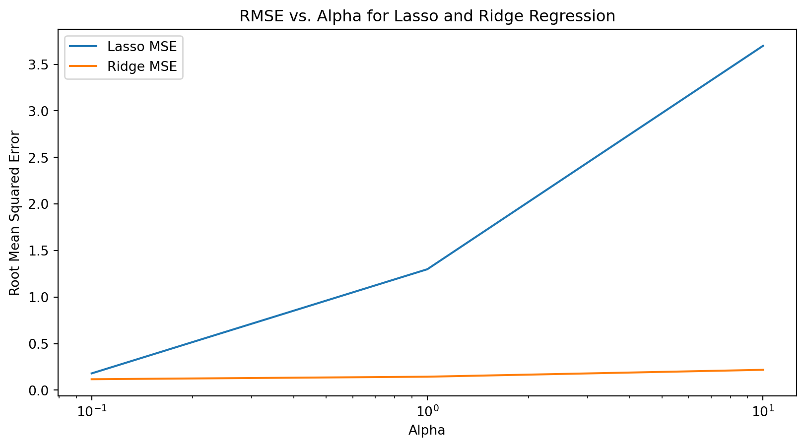
- Create a plot that looks at the alpha against the MSE for both lasso and ridge regression.
# Visualize alphas against RMSE for lasso and ridge

# Initialize lists to append data into
rmse_lasso = []
rmse_ridge = []

# Define alpha values to iterate over
alphas = [0.1,1,10]

# Create and fit a lasso and ridge model for each predefined alpha
for alpha in alphas:
    lasso = Lasso(alpha=alpha)
    ridge = Ridge(alpha=alpha)

    lasso.fit(X_train, y_train)
    ridge.fit(X_train, y_train)

    # Calculate rmse for both models
    rmse_lasso.append(np.sqrt(mean_squared_error(y_test, lasso.predict(X_test))))
    rmse_ridge.append(np.sqrt(mean_squared_error(y_test, ridge.predict(X_test))))

# Create plot of MSE again alpha values
plt.figure(figsize=(10, 5))
plt.plot(alphas, rmse_lasso, label='Lasso MSE')
plt.plot(alphas, rmse_ridge, label='Ridge MSE')
plt.xscale('log')
plt.xlabel('Alpha')
plt.ylabel('Root Mean Squared Error')
plt.title('RMSE vs. Alpha for Lasso and Ridge Regression')
plt.legend()
plt.show()
- Create an interactive plot (for both lasso and ridge) that allows you to adjust alpha to see how the actual vs predicted values are changing.
# Create function to run model and create plot

def update_alphas(alpha, model_type):

    # Condition to allow user to select different models
    if model_type == 'Lasso':
        model = Lasso(alpha=alpha)
    else:
        model = Ridge(alpha=alpha)

    # Fit and predict model
    model.fit(X_train, y_train)
    y_pred = model.predict(X_test)

    # Calculate model metrics
    rmse = np.sqrt(mean_squared_error(y_test, y_pred))
    r2 = r2_score(y_test, y_pred)

    # Create plot of predicted values against actual values with line of best fit
    plt.figure(figsize=(10, 5))
    # Add predicted and actual values
    plt.scatter(y_test, y_pred, color='blue', alpha=0.5, label=f'Predictions (alpha={alpha})')
    # Add line of best fit
    plt.plot([y_test.min(), y_test.max()], [y_test.min(), y_test.max()], 'k--', lw=2)
    plt.title(f'{model_type} Regression: Predictions vs Actual (alpha={alpha})')
    plt.xlabel('Actual Values')
    plt.ylabel('Predicted Values')
    plt.legend()
    # Adjust the position and aesthetics of the metric box
    plt.figtext(0.5, -0.05, f'MSE: {rmse:.2f}, R²: {r2:.2f}', ha="center", fontsize=12, bbox={"facecolor":"orange", "alpha":0.5, "pad":5})
    plt.show()

# Create interactive widgets

# Create alpha slider for choosing alpha value
alpha_slider = FloatLogSlider(value= 0 , base=10, min=-3, max=3, step=0.1, description='Pick an Alpha!')

# Create model selector for picking which model user wants to look at
model_selector = {'Lasso': 'Lasso', 'Ridge': 'Ridge'}

# Combine two widgets with model/plot output
interact(update_alphas, alpha=alpha_slider, model_type=model_selector)
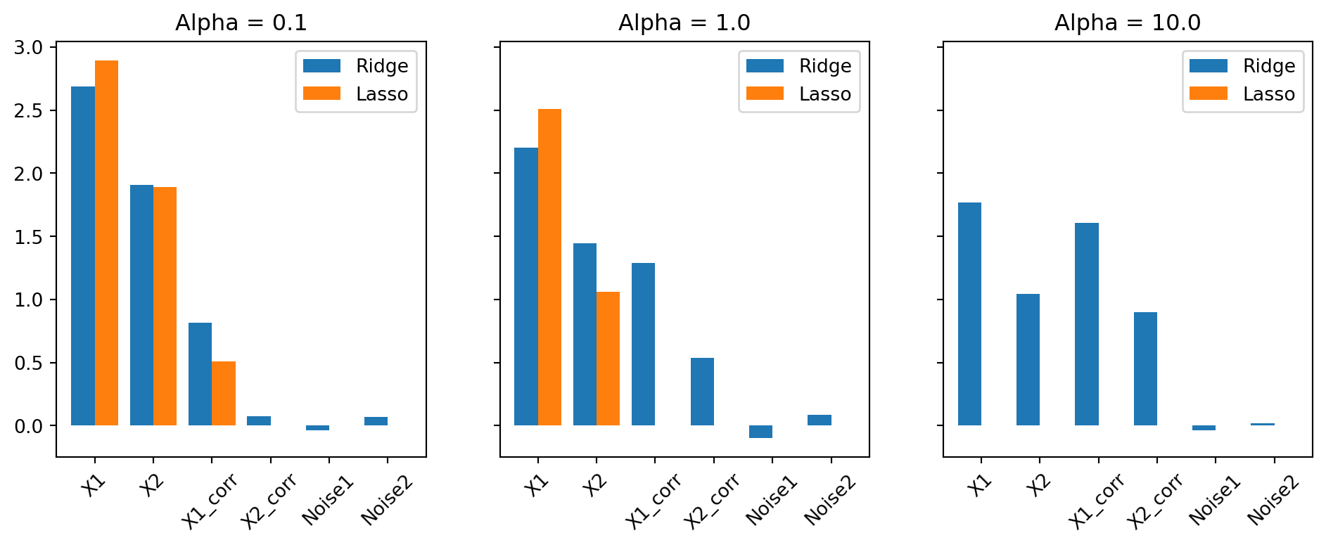
<function __main__.update_alphas(alpha, model_type)>- Create three different bar plots with the following guidelines: Each plot should represent a different alpha value: Alpha = 0.1, Alpha = 1, Alpha = 10 Each plot should show how both the ridge and lasso model performed The y axis should represent the six different variables:
X1,X2,X1_corr,X2_corr,Noise1,Noise2. The y axis should represent the coefficients
# Define alpha values to iterate over
alphas = [0.1, 1.0, 10.0]
data = []

# Create and fit ridge and lasso models and store coefficients in a new dataframe
for alpha in alphas:
    ridge = Ridge(alpha=alpha).fit(X_train, y_train)
    lasso = Lasso(alpha=alpha).fit(X_train, y_train)
    data.append(pd.DataFrame({
        'Ridge': ridge.coef_, # coef has as many indexes as there are variables
        'Lasso': lasso.coef_
    }, index=['X1', 'X2', 'X1_corr', 'X2_corr', 'Noise1', 'Noise2'])) # create feature names in new dataframe


# Create barplot to visualize how coefficients change across alpha values and models
fig, axes = plt.subplots(1, 3, figsize=(12, 4), sharey=True)
for i, df in enumerate(data):
    df.plot.bar(ax=axes[i], width= 0.8)
    axes[i].set_title(f'Alpha = {alphas[i]}')
    axes[i].set_xticklabels(df.index, rotation=45)

plt.show()